
By Kishan Sharma
Postgres is one of the most widely used open source databases in the world. At GOJEK, a lot of our products depend on Postgres as well. However, when you’re a building and operating a Super App at scale, the volume of data passing through the pipelines can slow down even the most efficient systems.
Sometimes, we witness degraded performance on Postgres too. That’s not a sustainable thing for a startup like GOJEK.
We needed to optimise things to enhance performance. So we targeted the optimizer.
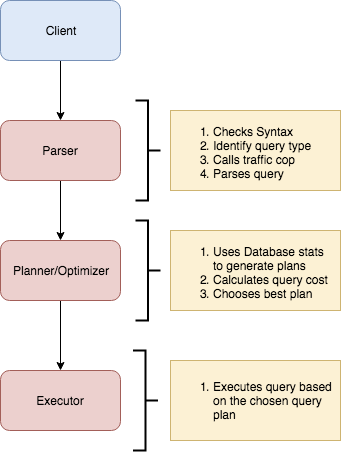
The optimizer is the brain of the database, which interprets queries and determines the fastest method of execution. A single query optimization technique can increase database performance drastically.
This post outlines how to analyse Postgres performance using tools such as EXPLAIN and ANALYZE (which Postgres provides).
Meet EXPLAIN & ANALYZE
EXPLAIN gives an exact breakdown of a query. The execution plan is based on the statistics about the table, and it identifies the most efficient path to the data. This takes different database paradigms (such as indexes) into consideration. EXPLAIN only guesses a plan that it thinks it will execute.
This is where ANALYZE comes into the picture. ANALYZE basically runs a query to find the processing time to execute a query.
To quickly summarise, EXPLAIN and ANALYZE commands help improve database performance in Postgres by:
a) Displaying the execution plan that the PostgreSQL planner generates for the supplied statement
b) Actually running the command to show the run time.
Finding the framework
Let’s consider we have a table named schemes.
EXPLAIN SELECT * FROM schemes;
QUERY PLAN | Seq Scan on schemes (cost=0.00..64 rows=328 width=479)
SELECT * FROM pg_class where relname = 'schemes';
pg_class has the metadata about the tables.
Cost in the query plan is calculated using the following formula
COST = (disk read pages * seq_page_cost) + (rows scanned * cpu_tuple_cost).
- Disk read pages and rows scanned are the properties of
pg_class. - Seq page cost is the estimated cost of disk read fetch.
- Cpu tuple cost is the estimated cost of processing each row.
e.g. COST (54 * 1.0) + (1000 * .01) = 64
Let’s see how the query plan changes when we apply filters in the select statement.
EXPLAIN SELECT * FROM schemes WHERE status = ‘active’;
QUERY PLAN | Seq Scan on schemes (cost=0.00..66.50 rows=960 width=384) Filter: ((status)::text = ‘active’::text)
The estimated cost here is higher than the previous query, this is because Postgres is performing a seq scan over 1000 rows first and then filtering out the rows based on the WHEREclause.
Planner cost constants
The cost variables described in this section are measured on an arbitrary scale. Only their relative values matter, hence scaling them all up or down by the same factor will result in no change in the planner’s choices. By default, these cost variables are based on the cost of sequential page fetches; that is, seq_page_cost is conventionally set to 1.0 and the other cost variables are set with reference to that. But you can use a different scale if you prefer, such as actual execution times in milliseconds on a particular machine.
Unfortunately, there is no well-defined method for determining ideal values for the cost variables. They are best treated as averages over the entire mix of queries that a particular installation will receive. This means that changing them on the basis of just a few experiments is very risky. (Refer planner cost constants).
EXPLAIN SELECT schemes.rules FROM scheme_rules JOIN schemes ON (scheme_rules.scheme_id = schemes.id ) where scheme_name = 'weekend_scheme';
The query planner sometimes decides to use a two-step plan. The reason for using two-plan node is the first plan sorts the row locations identified by the index into physical order before reading them, and the other plan actually fetches those rows from the table.
Down to the nuts and bolts
The first plan which does the sorting is called Bitmap scan.
Most common occurring matches are scanned using the seq scan and the least common matches are scanned using index scan, anything in between is scanned using bitmap heap scan followed by an index scan. One of the reasons for this is that the random I/O is very slow as compared to sequential I/O. This is all driven by analysing statistics.
Bitmap heap scan
A bitmap heap scan is like a seq scan — the difference being, rather than visiting every disk page, it scans ANDs and ORs of the applicable index together and only visits the disk pages it needs to visit. This is different from index scan where the index is visited row by row in order, which results in disk pages being visited multiple times. A bitmap scan will sequentially open a short list of disk pages and grab every applicable row in each one.
Sequential scan vs index scan
There are cases where a sequential scan is faster than an index scan. When reading data from a disk, a sequential method is usually faster than reading in random order. This is because an index scan requires several I/O for each row which includes looking up a row in the index, and based on that, looking up and retrieving the row from memory(heap). On the other hand, a sequential scan requires a single I/O operation to retrieve more than one block containing multiple rows.
Query plan on JOINS
The optimizer needs to pick the correct join algorithm when there are multiple tables to be joined in the select statement. Postgres uses three different kinds of join algorithms based on the type of join we are using.
Let’s dive in
Nested Loop: Here the planner can use either sequential scan or index scan for each of the elements in the first table. The planner uses a sequential scan when the second table is small. The basic logic of choosing between a sequential scan and index scan applies here too.
Hash Join: In this algorithm, the planner creates a hash table of the smaller table on the join key. The larger table is then scanned, searching the hash table for the rows which meet the join condition. This requires a lot of memory to store the hash table in the first place.
Merge Join: This is similar to merge sort algorithm. Here the planner sorts both the tables to be joined on the join attribute. The tables are then scanned in parallel to find the matching values.
Further reading on how we can use Explain/Analyze with join statements here
Postgres performance tuning is a complicated task. The complexity comes in identifying the appropriate ‘tunable’ from the many tools that Postgres provides. As you might have now guessed, there is no silver bullet to solving performance issues in Postgres — it’s the use case which dictates the tuning requirements.
The topics we covered here are about identifying problems and stats. You can read about how we can use this information for a solution to optimise Postgres, here:
The Postgres Performance Tuning Manual: Indexes
How to modify and improve query times in Postgres with the help of indexes.
blog.gojekengineering.com
Hope this helped. Keep following the blog for more updates!
#DYK that besides building a Super App, we also spend a good chunk of our time on learning and development? Working at GOJEK is as much about acquiring and sharing knowledge as it is about building cool things. Want to be part of this culture of growth? Well, we’re hiring, so head over to gojek.jobs and grab the opportunity to redefine on-demand platforms. And learn something new too.